Theoretical Background on FRFT

We have prepared a comprehensive tutorial on the theory and applications of the Fractional Fourier Transform (FRFT) in sound synthesis and processing, which we highly recommend going through before diving into the implementation details of this package:

In this post, we will briefly summarize the key concepts of the FRFT and then focus on the specific methods and implementation details of our real-time Max external and Max for Live device.

FRFT Recap

What is the FRFT?

As discussed in the tutorial linked above, the FRFT can be thought of as a rotation in a conceptual 2D time-frequency plane.

Where the standard Fourier Transform (FT) corresponds to 90-degree rotations in this plane (e.g. from time to frequency domain), the FRFT allows for arbitrary angles of rotation, controlled by the parameter α.

That means that the FRFT can produce representations that are intermediate between the time and frequency domains.

The location of the output in the time-frequency plane depends on the value of α (called the fractional order or rotation factor).

Special Cases

For special integer values of α, the FRFT reduces to familiar operations:

α value	Operation
0	Identity — signal is unchanged
1	Standard Fourier Transform
2	Time reversal
3	Inverse Fourier Transform

Inverse Operation

Unlike the standard FT, which has a dedicated inverse operation, the FRFT is self-invertible: applying the FRFT with a negative α undoes the transformation:

\[x[n] \xrightarrow{\mathcal{F}^{\alpha}} X[k] \xrightarrow{\mathcal{F}^{-\alpha}} x[n]\]

Index Additivity

The index additivity property of the FRFT states that applying two FRFTs in sequence with angles α₁ and α₂ is equivalent to applying a single FRFT with the sum of those angles:

\[\mathcal{F}^{\alpha_2} \circ \mathcal{F}^{\alpha_1} = \mathcal{F}^{\alpha_1 + \alpha_2}\]

Note that this essentially implies that the order of the transforms does not matter, as long as the total angle is the same:

\[\mathcal{F}^{\alpha_2} \circ \mathcal{F}^{\alpha_1} = \mathcal{F}^{\alpha_1} \circ \mathcal{F}^{\alpha_2}\]

Complex-Valued Output

Hence, if we start an audio signal (i.e. a real-valued time-domain waveform) and apply the FRFT with a non-integer α, we get a complex-valued output that contains both magnitude and phase information. We can then manipulate this output in various ways (e.g. apply filters, perform convolution, multiply with another signal) and then apply the inverse FRFT (i.e. FRFT with -α) to return to the time domain, resulting in a transformed audio signal that incorporates the effects of our manipulations in the fractional domain.

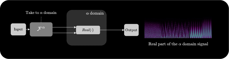
\[x[n] \xrightarrow{\mathcal{F}^{\alpha}} X[k] \xrightarrow{\text{Manipulation}} \tilde{X}[k] \xrightarrow{\mathcal{F}^{-\alpha}} \tilde{x}[n]\]

While this is the most straightforward way to use the FRFT for audio processing, we can also directly output the complex-valued result of the FRFT without applying an inverse transform. In such cases, we can take the real part of the output and use it as an audio signal directly.

\[x[n] \xrightarrow{\mathcal{F}^{\alpha}} X[k] \xrightarrow{\operatorname{Re}} \operatorname{Re}(X[k])\]

Windowing and Overlap

FRFT is not a sample-wise operation. Similar to spectral processing techniques like the Short-Time Fourier Transform (STFT), to process longer audio signals in real-time, we apply the FRFT to windowed segments of the input signal with a certain amount of overlap between consecutive windows.

The choice of window size, overlap, and windowing function (e.g. Hann, rectangular) can significantly affect the resulting sound, as they determine how the chirp structures evolve and blend across time.

FRFT External Overview

To be able to use the FRFT in real-time audio processing and synthesis contexts, we have developed a dedicated Max external called frft.

The external has been designed to work within Max’s pfft~ framework.

Here is a simple patch that demonstrates how to use the frft external within a pfft~ patcher environment:

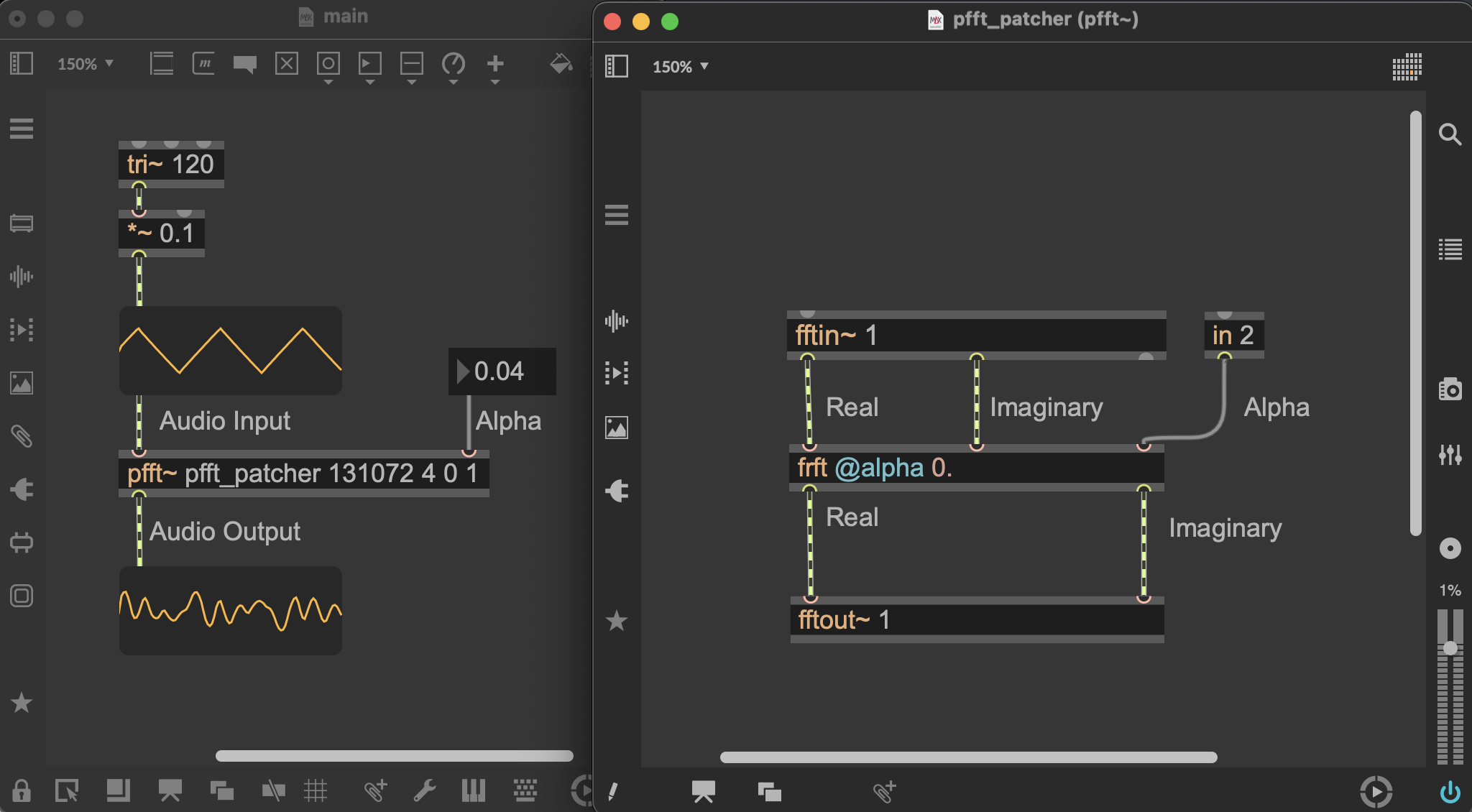
the arguments for pfft~ are as follows:

• The first argument (e.g. pfft_patcher) is the name of the subpatcher that contains the processing chain (i.e. the frft external in this case).
• The second argument (e.g. 131072) is the window size, which must be a power of two (otherwise will be rounded to the nearest power of two).
• The third argument (e.g. 4) is the number of overlap segments, which determines how much the windows overlap with each other (e.g. 4 means 75% overlap).
• The fourth argument should be set to 0
• The fifth argument should be set to 1 to signify that we work with the full spectrum (this is the correct structure required by FRFT). That said, you can also set it to 0 to work with the half spectrum to try out different textures.

pfft~ is a powerful tool in Max for performing spectral processing on audio signals. pfft~ has built-in support for specialized windowing, overlap, and buffering mechanisms that allow for efficient real-time processing of audio streams in the frequency domain. Of course, the FRFT is not a standard spectral processing technique, however, certain properties of the FRFT allow us to in fact leverage the pfft~ framework for our purposes. Below we discuss this in more detail.

Why does FRFT work within pfft~?

For the intended applications using FRFT, we typically work with windowed segments of audio signals, generally in an overlapped manner.

While the pfft~ environments, facilitates overlap-add processing and windowing, it provides the users with the FT of windowed segments and also requires the results to be provided in the same format (i.e. windowed segments in the frequency domain).

So why is it possible to use the FRFT within this framework?

The answer lies in one of the main mathematical properties of the FRFT that we’ve discussed previously (index additivity).

Let’s look at the example patch above. In this patch, a given window of audio goes through the following chain of operations:

1. The input audio signal is windowed and transformed to the frequency domain by fftin~ (i.e. FT).
2. The output of fftin~ is then fed into the frft external, which applies the FRFT with a specified α to the input.
3. The output of the frft external is then fed into fftout~, which applies the inverse FT to return to the time domain and outputs the processed audio signal.

\[x_w[n] \xrightarrow{\text{FT}} X[k] \xrightarrow{\mathcal{F}^{\alpha}} \tilde{X}[k] \xrightarrow{\text{IFT}} \tilde{x}_w[n]\]

Now remember that FT and IFT are equivalent to FRFTs with specific α values ($\text{FT} = \mathcal{F}^{1}$ and $\text{IFT} = \mathcal{F}^{-1}$).

Therefore, the above chain of operations can be rewritten as:

\[x_w[n] \xrightarrow{\mathcal{F}^{1} \circ \mathcal{F}^{\alpha} \circ \mathcal{F}^{-1}} \tilde{x}_w[n]\]

Which using the index additivity property of the FRFT can be simplified to:

\[x_w[n] \xrightarrow{\mathcal{F}^{1+\alpha-1}=\mathcal{F}^{\alpha}} \tilde{x}_w[n]\]

So, while all data within the pfft~ environment is technically provided in the frequency domain, the fftin~/fftout~ operations effectively cancel each other out; this is as if we had directly applied the FRFT to the windowed audio segment in the time domain!

Limitations and Considerations

While pfft~ simplifies the windowing/overlap management, it also imposes certain constraints on how we can use the FRFT.

First, the pfft~ framework only works with window sizes that are powers of two, which may limit the range of window sizes we can use for FRFT processing.

Second, while we can dynamically modify the window settings, everytime we do so, the pfft~ environment needs to be re-initialized, which can cause audio dropouts.

Thirdly, the pfft~ framework involves two FFT operations (fftin~ and fftout~) in the processing chain, which for our purposes are essentially redundant due to the index additivity property of the FRFT. This means that we are doing more computations than necessary, which can increase the CPU load and reduce the efficiency of our processing.

We are planning to develop an alternative FRFT external that does not rely on the pfft~ framework, which will allow us to bypass these limitations and optimize the processing chain for FRFT-specific applications. However, in such case, all operations will be handled within the external, meaning that the underlying chain of operations will not be exposed to the user, hence won’t be modifiable within max (can only be modified by changing the source code of the external itself). As such, we believe the current pfft~-based implementation strikes a good balance between flexibility and usability for a wide range of applications, while also allowing users to experiment with the FRFT in real-time audio contexts without needing to worry about the underlying complexities of the transform.

Applications

At the end of the tutorial linked above, we discussed several potential applications of the FRFT in sound synthesis and processing contexts.

Here, we discuss how our external can be used to implement these applications in real-time within Max/MSP.

These methods have been implemented both as standalone Max patches as well as Max for Live devices. After installation:

• Max patches in Max 8 (or 9)/Packages/FRFT/standalone folder
• Max for Live devices in the Max 8 (or 9)/Packages/FRFT/m4l folder.

In the following sections, we will first focus on the standalone Max patches. Subsequently, we’ll have a quick overview of the Max for Live devices and how they can be used within Ableton Live.

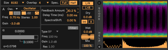
A general note about all the systhesis methods: The resulting sounds are extremely sensitive to the choice of α. Even miniscule changes in α can lead to significant changes in the output timbre. In the standalone patches, we suggest entering α values with high precision to be able to explore the full range of textures that the FRFT can produce. In the Max for Live devices, we have implemented a high-precision α control interface that allows for fine-grained adjustments to the parameter in real-time (More on this later in the Max for Live section).

A few things to try out in all the following methods:

• In the standalone Max patches, we have implemented a simple modulation source for dynamically modulating the α parameter over time. You can use different modulation shapes at different rates/depths to explore a wide range of dynamic behaviors in the resulting sounds.
• Whenever using an oscillator input, we suggest trying different frequencies for the input oscillator. Try sub-audio frequencies (< 20 Hz) and explore the impact on the generated textures.
• Change the Full/Half spectrum flag and see how it affects the resulting sound

α-synthesis and α-processing

Method

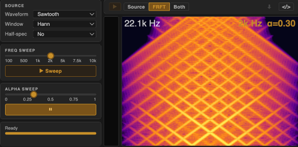
For α-synthesis, we apply a single FRFT transformation to a simple oscillator (e.g. sine, square, triangle, sawtooth) to generate complex, dynamically evolving sounds from scratch.

Here, each pure tone at a non-integer α produces chirp-like textures — horizontal lines in the time domain becomes a set of diagonal structures in the spectrogram. The spectral richness of the input directly determines the complexity of the output: harmonically richer waveforms (e.g. sawtooth) produce denser, more layered textures.

α-processing applies the same FRFT chain to an existing audio recording or live input. Here more complex and dynamic source material can produce a wider variety of textures.

For $\alpha = 0$, the output is identical to the input. For $\alpha = 2$, the output is the time-reversed version of the input. (Try large windows with $\alpha$ close to 2 for interesting time-reversal effects—most perceptible in $\alpha$-processing).

Demo

Here is a demo of α-synthesis:

Change the resolution of the videos to 1080p to be able to better see the details

And here is a demo of α-processing applied to a number of different source materials:

An interesting setting to try out in α-processing: Set the alpha value close to FT (i.e. 0.99 or -0.99), and also use low source frequencies (even sub-audio frequencies). This results in very interesting rhythmic textures. Here is a demo:

In the last demo, we can clear see that having continuous control over Overlap Add, Window Size, and Window Type parameters can be very useful for modifying the textures without interruption. This is the main reason why we are working on an alternative implementation of the FRFT external that does not rely on pfft~ and allows for real-time control over these parameters without needing to re-initialize the processing environment (which causes audio dropouts in the current implementation).

α-Convolution

Method

α-Convolution transforms two signals to the same fractional domain ($\mathcal{F}^{\alpha}$), multiplies them, and then applies the inverse FRFT ($\mathcal{F}^{-\alpha}$) to return to the time domain:

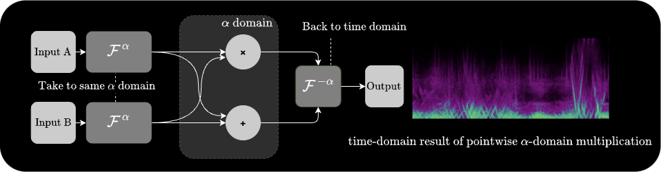
At α = 1 this is identical to standard frequency-domain convolution. At other values of α, the convolution is performed along a rotated axis in the time-frequency plane, which can impose the spectral envelope of one signal onto the chirp structure of the other in ways that standard convolution cannot.

Demo

Here is a demo of convolving a sine wave with a square wave in the fractional domain:

Here is a demo of convolving a looping recording of a voice with un-synced version of itself in the fractional domain:

α-Filtering

Method

α-Filtering is very similar to α-Convolution, but instead of convolving two signals, we apply a filter response H[k] pointwise in the fractional domain representation of a single signal:

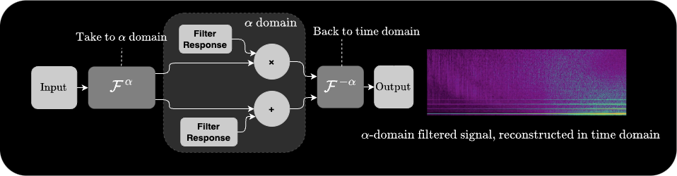
At α = 1 this reduces to standard frequency-domain filtering. At other values of α, the filter mask is applied along a rotated axis — enabling filter shapes that would be impossible in the standard frequency domain, such as filtering out specific chirp rates while preserving others.

In the max patch, we filter white noise and then feed it to the same α-convolution chain to further modify the texture. Alternatively, you can calculate the complex response of the filter and apply it directly in the fractional domain (this is what we do in the Max for Live device).

Demo

Here is a demo of α-filtering applied to a vocal recording:

α-RM (Ring Modulation)

Method

α-Ring Modulation transforms two independent signals into different fractional domains (α₁ and α₂), multiplies them pointwise in those domains, and outputs the real part of the result directly — without applying an inverse FRFT:

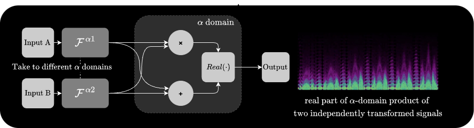
At α₁ = α₂ = 0, this reduces to standard time-domain ring modulation (i.e. pointwise multiplication of two signals, in an overlap-add manner).

Try different combinations of α₁ and α₂ to see how the resulting textures change. Specifically, try out combinations where the pairs are correlated (e.g. $\alpha_1 = 0.5$ and $\alpha_2 = 0.5$) vs. uncorrelated (e.g. $\alpha_1 + \alpha_2 = 0, 1, 2$) to see how the relationship between the two rotation factors affects the resulting sound.

Demo

Here is a demo of ring modulating two triangle wave oscillators with different frequencies in the fractional domain:

Here is a demo of ring modulating a guitar recording with a sine wave in the fractional domain:

Other Methods

Above methods are just a few examples of how the FRFT can be used for sound synthesis and processing.

We encourage you to experiment with the frft external and come up with your own creative applications of the FRFT in real-time audio contexts.

As an example, here are two demos of a more complex patch that uses a FRFT operation in a feedback loop (in the pfft environment) to create evolving textures from a simple input signal:

MaxForLive Integration

All of the above methods have also been implemented as Max for Live devices that can be used within Ableton Live.

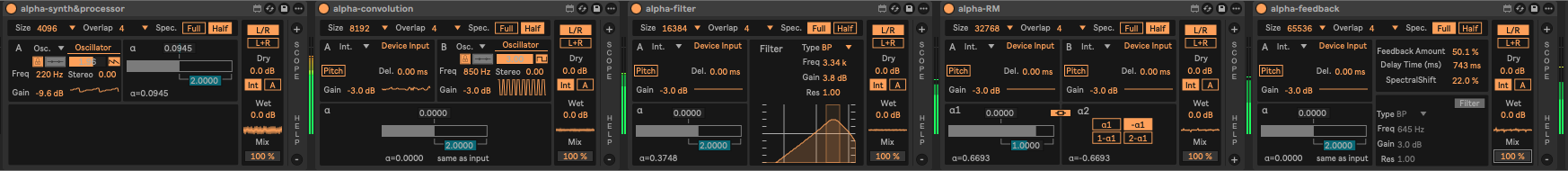
These devices are accessible in the Max 8 (or 9)/Packages/FRFT/m4l folder after installation:

• alpha-synth&processor.amxd
• alpha-convolution.amxd
• alpha-filter.amxd
• alpha-RM.amxd
• alpha-feedback.amxd

The underlying FRFT operations in these devices are the same as in the standalone Max patches. The main difference is the Max for Live interface, which allows for easier integration into Ableton Live projects and provides a more user-friendly control surface for the parameters.

Overview of Interface

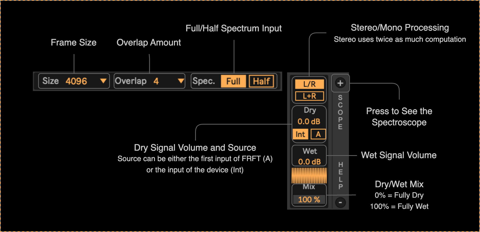
Windowing and Mix Controls (available in all devices)

Input Audio Routing (available in all devices)

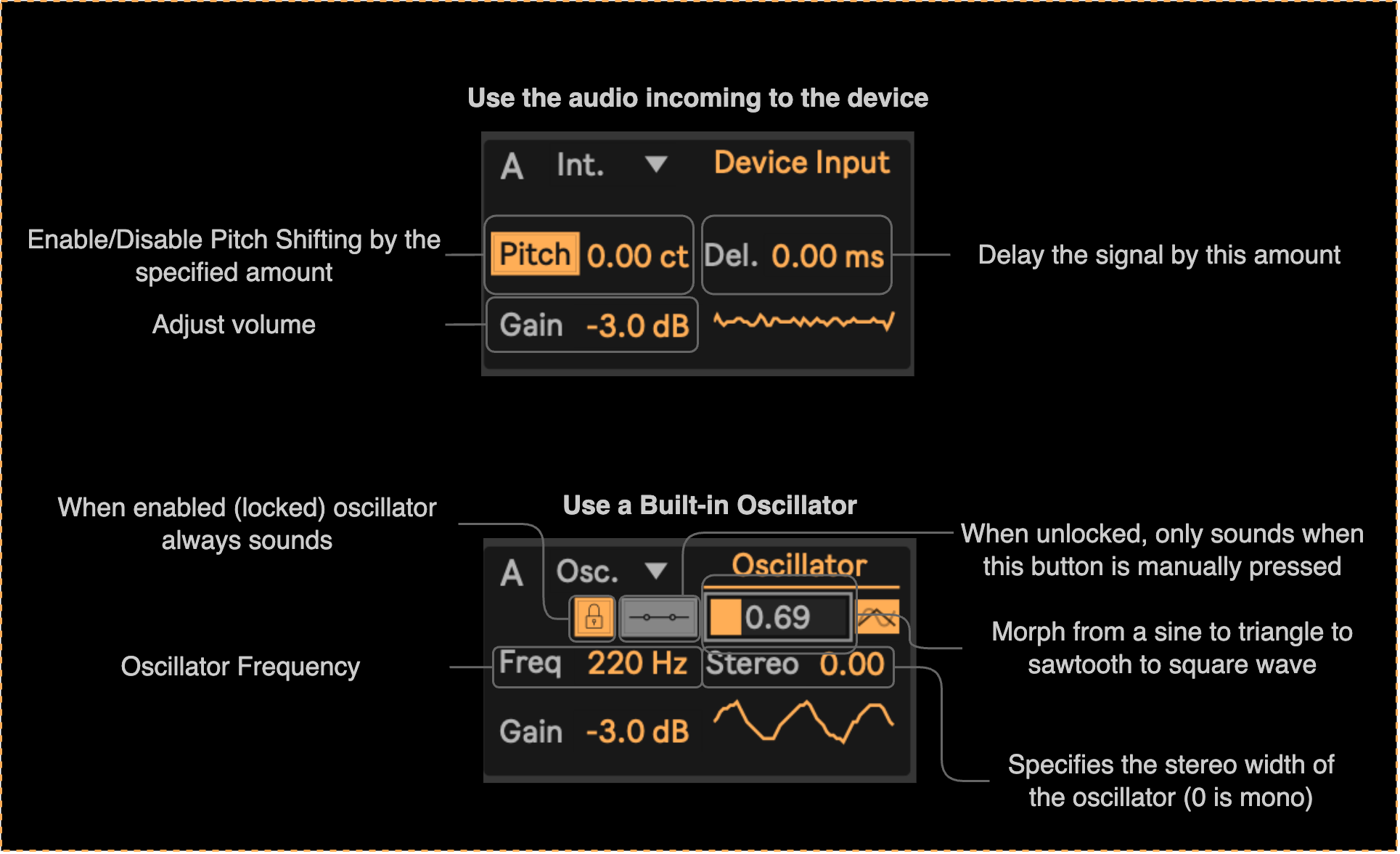
Depending on the device, one or two audio inputs are required for the processing. These sources can be set via the A/B panels.

The audio can come either from the track on which the device is loaded (called ‘internal’ source) or from a built-in oscillator (called ‘osc’):

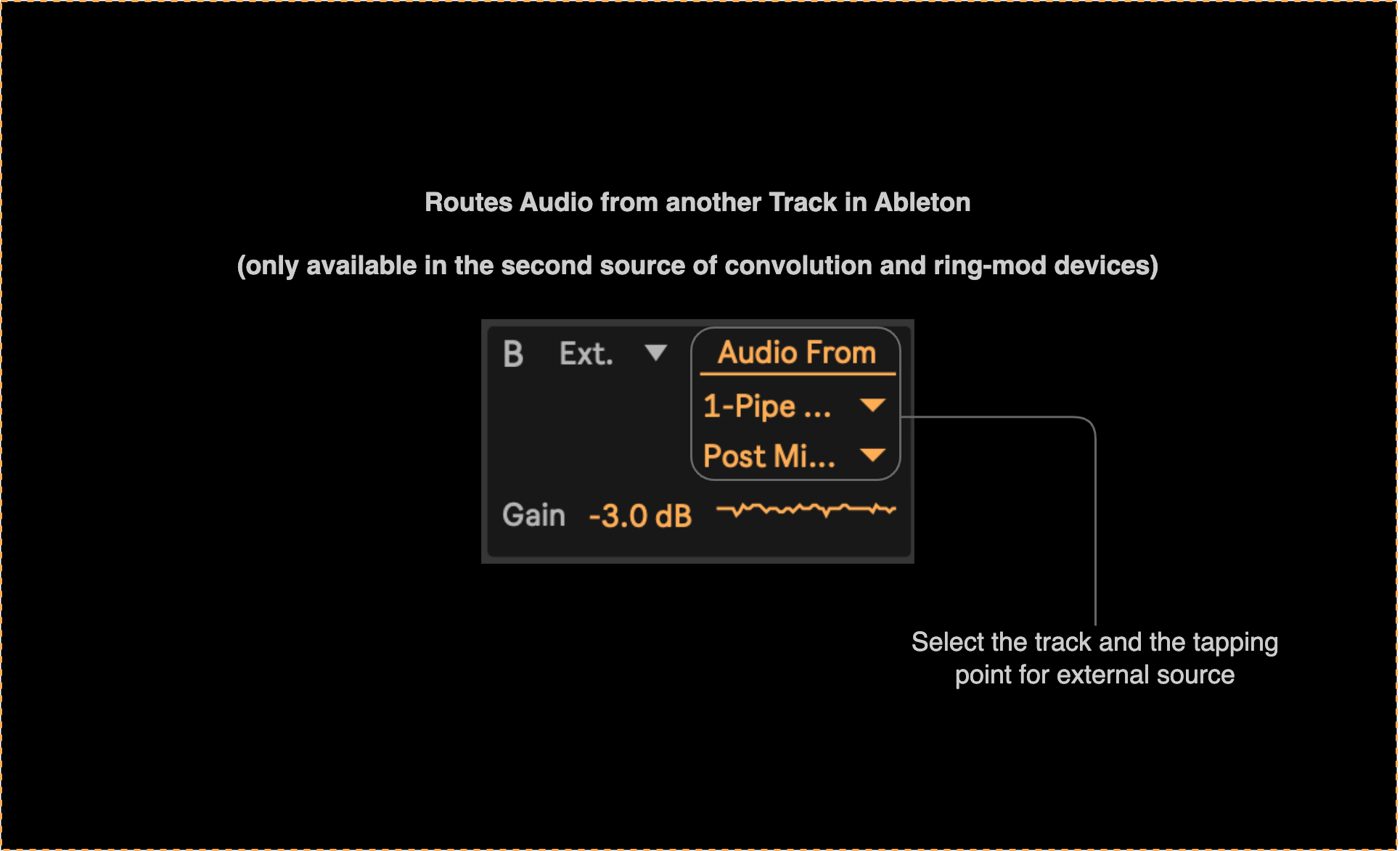
Moreover, in the case of α-convolution and α-RM devices, the second source can also be routed from anywhere in the Live set using the ‘external’ option:

$\alpha$ Control Panels

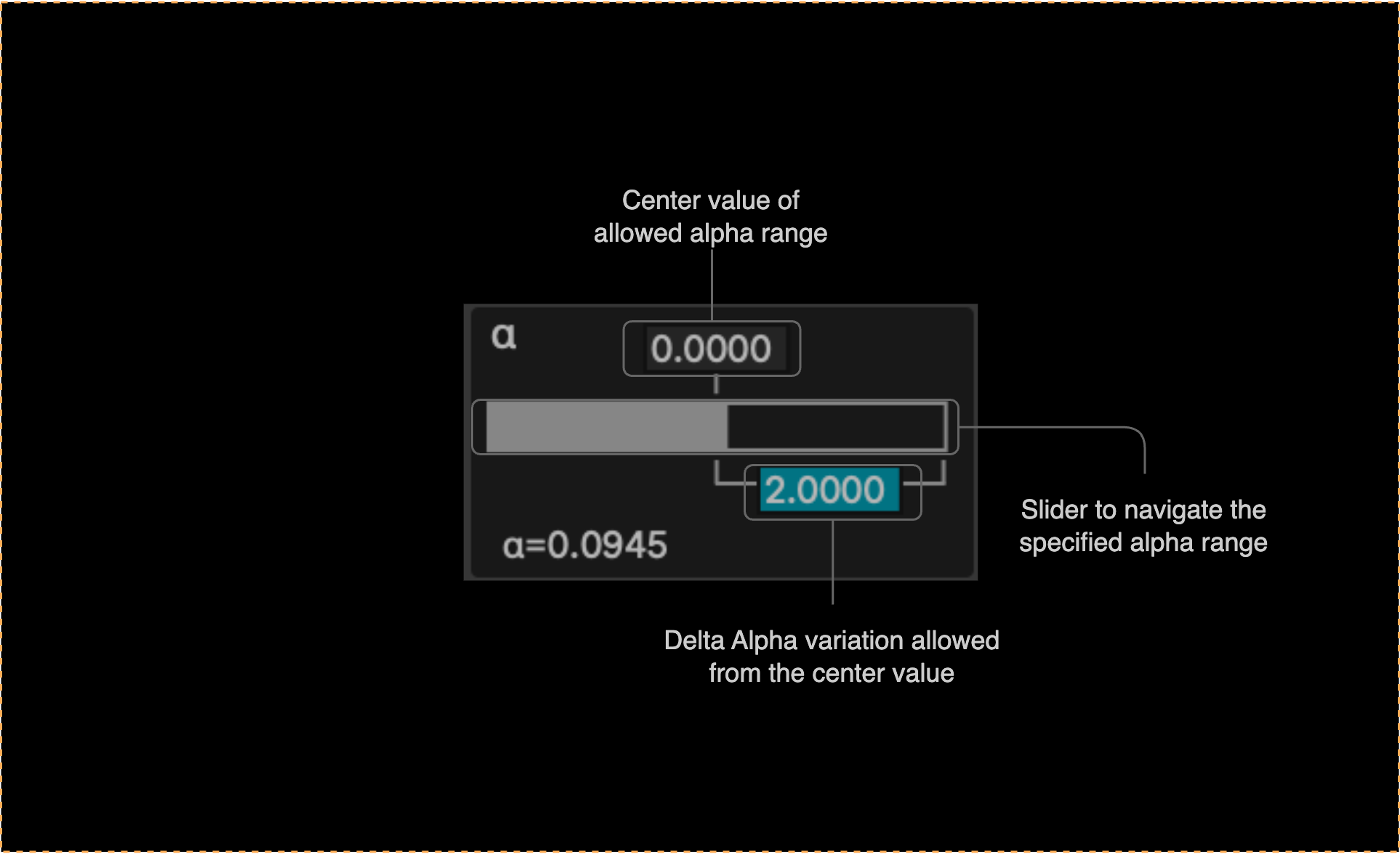
For controlling the α parameters, we have implemented a custom control interface that allows for high-precision adjustments to the α values in real-time.

Instead of specifying a single α value, the user can specify a range of allowed α values (by setting the center and width of the range), and then a dedicated slider is used to smoothly navigate within that range.

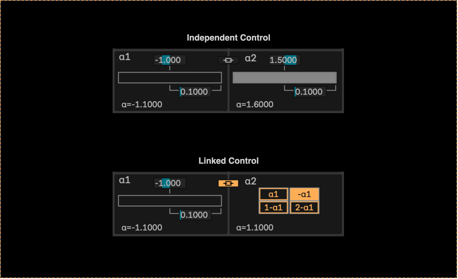
In the case of α-RM, where we have two independent α parameters, the interface allows for controlling the ranges of both parameters independently or linking the second parameter to the first one with a specified offset (e.g. $\alpha_2 = \alpha_1 + 1.0$)

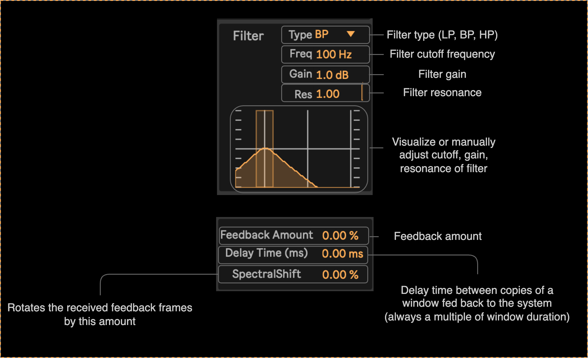
Feedback and Filter Controls

In the α-feedback and α-filter devices, we have a panel for controlling the filter parameters:

Moreover, in the α-feedback device, we have a dedicated panel for controlling the feedback amount: