Overview
In this tutorial, we will go over an innovative synthesis method proposed by Gutiérrez et al.:
Fractional Fourier Sound Synthesis
Proceedings of the International Computer Music Conference (ICMC) · 2025Abstract
This paper explores the innovative application of the Fractional Fourier Transform (FrFT) in sound synthesis, highlighting its potential to redefine time-frequency analysis in audio processing. As an extension of the classical Fourier Transform, the FrFT introduces fractional order parameters, enabling a continuous interpolation between time and frequency domains and unlocking unprecedented flexibility in signal manipulation. Crucially, the FrFT also opens the possibility of directly synthesizing sounds in the alpha-domain, providing a unique framework for creating timbral and dynamic characteristics unattainable through conventional methods. This work delves into the mathematical principles of the FrFT, its historical evolution, and its capabilities for synthesizing complex audio textures. Through experimental analyses, we showcase novel sound design techniques, such as alpha-synthesis and alpha-filtering, which leverage the FrFT’s time-frequency rotation properties to produce innovative sonic results. The findings affirm the FrFT’s value as a transformative tool for composers, sound designers, and researchers seeking to push the boundaries of auditory creativity.
BibTeX
@inproceedings{gutierrez2025fractionalfouriersoundsynthesis,
  title = {Fractional Fourier Sound Synthesis},
  author = {Guti{\'e}rrez, Esteban and C{\'a}diz, Rodrigo and Long, Carlos Sing and Font, Frederic and Serra, Xavier},
  year = {2025},
  eprint = {2506.09189},
  archiveprefix = {arXiv},
  primaryclass = {cs.SD},
  booktitle = {Proceedings of the International Computer Music Conference (ICMC)}
}
We will start with a quick refresher on the Fourier Transform (FT).
Subsequently, we introduce the concept of the Fractional Fourier Transform (FRFT) and discuss its properties and how it relates to the FT.
Then, we will explore how to utilize the FRFT for sound synthesis and processing.
Fourier Transform
Let’s start with a quick refresher on the Fourier Transform (FT).
What is Fourier Transform?
The FT is a mathematical transformation that decomposes a signal into its constituent frequencies.
Basicaly, FT transforms a time-domain signal into a frequency-domain representation.
For instance, if you have a pure tone at 1000 Hz, FT results in a representation such as the following:
In this repesentation, the x-axis corresponds to frequency, and the y-axis corresponds to the amplitude of each frequency component. Now, if you add harmonics to the pure tone, you will get a more complex spectrum (try it out by changing the waveform type in the demo above).
FT results in a complex-valued signal, here we are only showing the magnitude of this complex signal for simplicity.
When we perform FT on a real signal (like an audio signal), we get a spectrum that is symmetric (as in the example above). In such cases, commonly we work with the positive frequencies (the right half of the spectrum) since the negative frequencies are just a mirror image of the positive ones. That said, in this tutorial, we will be working with the full spectrum. This will be important when we discuss Fractional Fourier Transform (FRFT) later on.
Fourier Transform for Synthesis and Processing
There are many applications of the FT in sound synthesis and processing.
Most common methods rely on the inversibility of the FT, which means that we can transform a signal to the frequency domain and also perform the inverse operation to get back to time domain.
\[x[n] \xrightarrow{\text{FT}} X[k] \xrightarrow{\text{IFT}} x[n]\]With this property, we can synthesize/process sounds by applying IFT to a spectrum created from scratch or a spectrum obtained from an existing signal,
\[Y[k] \xrightarrow{\text{IFT}} y[n]\] \[x[n] \xrightarrow{\text{FT}} X[k] \xrightarrow{\text{Manipulation}} \tilde{X}[k] \xrightarrow{\text{IFT}} \tilde{x}[n]\]The frequency-domain signals are generally complex-valued, which means that they have both a real part and an imaginary part. To ensure that the resulting time-domain signal is real-valued, the complex spectrum must satisfy the conjugate symmetry property, which states that the negative frequency components are the complex conjugate of the positive frequency components: \(X[-k] = X[k]^*\)
Treating Fourier Transform Components as Audio Signals
In the above examples, to listen to the spectrum, we applied the IFT to the complex spectrum to get back to the time domain.
However, it is also possible to listen to the real, imaginary parts of the complex spectrum directly without applying IFT.
\[x[n] \xrightarrow{\text{FT}} X[k] \xrightarrow{\text{Real Part}} \text{Re}\{X[k]\}\]or
\[x[n] \xrightarrow{\text{FT}} X[k] \xrightarrow{\text{Imaginary Part}} \text{Im}\{X[k]\}\]In other words, we treat the real or the imaginary component of the complex spectrum as an audio signal directly.
In the following demo, you can try out different waveforms and listen to the real (or imaginary) part of their Fourier Transform directly, while treating them as audio signals:
Try out different waveforms: sine, square, triangle, and sawtooth. In these cases, the resulting sound is a squence of clicks, as the Fourier Transform of these waveforms consists of a series of impulses at the harmonic frequencies.
When interacting with the demo, notice the X-axis transforming from frequency to time as soon as you play the sound. In the rest of this tutorial, we will be listening to the real part of any complex signal, whether obtained from the FT or any other operation.
Rotational Behavior of Fourier Transform
As discussed above, the FT transforms a signal from the time domain to the frequency domain. Likewise, there is an inverse operation called the Inverse Fourier Transform (IFT) that transforms a signal from the frequency domain back to the time domain.
\[x[n] \xrightarrow{\text{FT}} X[k] \xrightarrow{\text{IFT}} x[n]\]An interesting property of the FT is that if we apply the FT four times consecutively, you will get back to the original signal:
\[x[n] \xrightarrow{\text{FT}} X[k] \xrightarrow{\text{FT}} x[-n] \xrightarrow{\text{FT}} X[-k] \xrightarrow{\text{FT}} x[n]\]To conceptualize this, we can think of the time-frequency plane as a 2D space where the x-axis represents time and the y-axis represents frequency. As such, applying the FT corresponds to a 90-degree rotation in this plane. The following demo visualizes this rotational behavior of the FT:
Press on the waveforms to listen to the corresponding time-domain or frequency-domain signals
The waveforms at the frequency domain are the real part of the Fourier Transform.
To understand the impact of time reversal, use the “Freq sweep” input and also switch to “Spectrogram” visualization.
Fractional Fourier Transform
FRFT as a Generalization of Fourier Transform
We ended the previous section by mentioning that the Fourier Transform (FT) can be thought of as a rotation in a conceptual time-frequency plane.
That is, in this 2D conceptual space, a 90-degree rotation corresponds to a single application of the FT, and given its rotational behavior, applying the FT four times will bring you back to the original signal.
Now, the question is: Can we apply a rotation that is not necessarily 90 degrees? If so, what sort of intermediary sounds would be achieved?
This is exactly what the Fractional Fourier Transform (FRFT) allows us to do. The FRFT is a generalization of the FT that enables us to perform rotations by arbitrary angles in the time-frequency plane.
Here is an extended version of the previous demo that also allows for intermediate rotations using the FRFT:
Notice that in this demo (as opposed to the previous one), instead of showing angles of 0, 90, 180, and 270 degrees,
we are using integer values of 0, 1, 2, and 3 to represent the same angles.
This is because in the context of the FRFT, a rotation of 90 degrees corresponds to a value of 1.
We call this value the fractional order or rotation factor of the FRFT, and we typically denote it by the symbol $\alpha$ (alpha).
\(\text{Rotation Angle} = \alpha \times 90^\circ\)
Switch between the Waveform/Spectrogram tabs to visualize the waveforms or their spectral content at different rotation factors.
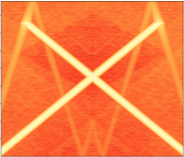
Looking at the spectrograms for a single static sine input, you can see that at non-integer values of $\alpha$ (i.e. in between the time and frequency domains), the resulting waveforms have a more complex structure. For instance:
A single tone (visible as a horizontal line in the time domain) is transformed into chirp-like structures (visible as multiple diagonal line in the spectrogram) at intermediate rotation factors.
Some Useful Properties of FRFT
In this section, we will go over some useful properties of the FRFT that are relevant to sound synthesis and processing.
We won’t get into the mathematical details of these properties, but we will provide some intuition and examples to illustrate them. (The paper on which this tutorial is based provides a rigorous mathematical treatment of these properties, so we encourage you to check it out for more details if you’re interested.)
Special Cases of FRFT
We have already discussed that the FRFT is a generalization of the FT, and as such, it has some special cases that correspond to specific values of the rotation factor $\alpha$:
- When $\alpha = 0$, the FRFT reduces to the identity operation, meaning that the output is the same as the input signal.
- When $\alpha = 1$, the FRFT reduces to the standard Fourier Transform
- When $\alpha = 2$, the FRFT corresponds to a reversal operation
- When $\alpha = 3$, the FRFT corresponds to an inverse Fourier Transform
The following demo illustrates these special cases applying the FRFT to a sine sweep input:
Inverting the FRFT
Remember that in the case of the FT, we had a dedicated inverse operation called the Inverse Fourier Transform (IFT) that allowed us to transform a signal from the frequency domain back to the time domain.
In the case of the FRFT, there is no separate inverse operation. Instead, the inverse of the FRFT is also a FRFT, but with a negative rotation factor.
\[x[n] \xrightarrow{\mathcal{F}^{\alpha}} X_\alpha[k] \xrightarrow{\mathcal{F}^{-\alpha}} x[n]\]A positive rotation factor $\alpha$ corresponds to a counter-clockwise rotation in the time-frequency plane, while a negative rotation factor corresponds to a clockwise rotation.
In the following demo, you can transform a signal into the alpha domain and then apply the inverse transformation to get back to the original signal:
Here you can see that the final output after $\alpha$ and $-\alpha$ transformations is almost identical to the original input signal.
In this demo, we visualize the error between the two paths. For a perfect mathematically accurate implementation of the FRFT, this error should be zero. However, in here, we are using a light-weight implementation of the FRFT which is highly optimized for real-time performance at the cost of some accuracy. Hence, the error is not exactly zero, but it is still very small and inaudible in most cases. That said, in pure mathematical terms, the error should be zero, and the original signal should be perfectly reconstructed after applying the FRFT and its inverse.
Index Additivity
The FRFT has an interesting property called index additivity, which states that if you apply two FRFTs with rotation factors $\alpha_1$ and $\alpha_2$ consecutively, it is equivalent to applying a single FRFT with a rotation factor that is the sum of the two individual rotation factors:
In the following demo, you can apply two consecutive FRFTs and observe the resulting waveforms and spectrograms at each step, as well as the final result of applying a single FRFT with the combined rotation factor:
Impact of Input Signals and $alpha$ on the Resulting Textures
The resulting sounds obtained from applying the FRFT to an input signal can vary greatly depending on the characteristics of the input signal and the chosen rotation factor $\alpha$.
In this part, we will see how the spectral content of a sound, as well as the choice of $\alpha$, can impact the resulting textures obtained from applying the FRFT.
To start with, let’s look at the following demo in which we use a sine sweep input signal and apply the FRFT with different values of $\alpha$ to observe the resulting waveforms and spectrograms:
The first observation here is that the spectral content of the textures in the right and left half of the time-frequency plane are mirrored versions of each other. Moreover, similar textures can be obtained in the top-right and bottom-right quadrants. With these observations in mind, for the remainder of this section, we will focus on the top-right quadrant of the time-frequency plane, which corresponds to fractional orders between 0 and 1 $(\alpha \in [0, 1])$.
In the following demo, for a specific input type, we render many different combinations of $\alpha$ and the input frequency content. We suggest interacting with the demo and exploring the impact of these parameters on the resulting textures.
Select the ‘BOTH’ option, to visualize and listen to the source and transformation concurrently. For now, we suggest not modifying the source panel (except for the source type)
We suggest the following steps to explore the impact of $\alpha$ and the input spectral content on the resulting textures:
- At a fixed value of $\alpha$, move the frequency slider to explore the impact of the input spectral content on the resulting textures.
- At a fixed input frequency, move the $\alpha$ slider to explore the impact of $\alpha$ on the resulting textures.
- Try out different waveforms (sine, square, triangle, and sawtooth) to explore the impact of the input waveform on the resulting textures.
Impact of Windowing
The way we’ve been applying the FRFT so far is by taking the entire input signal, applying the FRFT to it, and then listening to the resulting output.
That said, just like most spectral processing techniques, the FRFT can also be applied in a windowed manner, where we take a short segment of the input signal (called a window), apply the FRFT to that segment, and then move the window across the entire signal to process it in chunks.
To construct the final output, we can either concatenate the processed segments together (non-overlapping windows) or we can overlap and add the processed segments together (overlapping windows).
Window Size Vs. Chirp Speed
Let’s start with considering this example: Window-based FRFT of a long Sinusoidal signal with a fixed frequency.
The way we can apply FRFT, is either we apply it to the entire signal at once, or we can chop the signal into smaller non-overlapping segments and apply the FRFT to each segment separately.
Because the spectral content in each of the cases (regardless of the segment size) is the same (all containing a single horizontal line representing the frequency of the sine signal),
the resulting spectrograms look similar.
However, when we play each of the resulting outputs, the speed at which the textures evolve over time is different.
This can be observed in the following demo in which on the left we use a window size of 131072 samples and on the right we use half this size i.e. 32768 samples):
As you notice, while the spectral content look the same, the textures for the smaller window size (on the right) evolve faster over time compared to the larger window size (on the left).
The smearing of the spectrum on the write panel is due to the smaller window size, which results in a lower frequency resolution.
Overlapping Windows
We can also apply the FRFT in an overlapping manner, where we take overlapping segments of the input signal, apply the FRFT to each segment separately, and then overlap and add the processed segments together. In this case, you can clearly see that the chirp-like structures from one window bleed into the next window:
Change the overlap parameter to see the impact of different overlap amounts on the resulting textures.
Increasing it, results in faster textures with more chirp-like structures.
Effect of Windowing Functions
In these demos, we apply a Hann window to each segment before applying the FRFT, which helps to reduce spectral leakage and create smoother transitions between the segments when they are overlapped and added together. If you don’t apply any windowing function (i.e. use a rectangular window), you will get more abrupt transitions between the segments, which can result in additional chirp-like structures in the spectrograms.
Synthesis with FRFT
Basic Synthesis and Processing with FRFT
In fact, in many of the examples we have seen so far, we have been using the FRFT for synthesis and processing without explicitly mentioning it.
In these examples, we discussed how we can create (i.e. synthesize) quite complex dynamically evolving sounds by simply applying FRFT to simple signals such as a pure tone.
While for simplicity, we usually focused on pure tone inputs, we occasionally discussed that we can use more harmonically rich signals.
The following demo allows you to experiment with different input waveforms and listen to the resulting sound after applying FRFT to them.
Moreover, we can use the same processing chain for sound processing as well. That is, instead of synthesizing complex sounds from simple inputs, we can take an existing sound and apply FRFT to it to get a transformed version of the original sound.
Here are some example of processing audio recordings with FRFT:
The audio demos here correspond to the following freesound.org recordings: https://freesound.org/people/elzozo/sounds/613395/ and https://freesound.org/people/owstu/sounds/628817/ . Press the folder icon to try with your own audio files.
A Few Final Notes
Other Ways to Use FRFT for Synthesis/Processing
So far we just applied a single FRFT to a single source and listened to the real part of the resulting signal. However, there are many other ways to use the FRFT for synthesis and processing.
For exmaple, we can manipulate a signal in alpha domain and then apply the inverse FRFT to listen to the resulting sound directly in time domain.
\[x[n] \xrightarrow{\mathcal{F}^{\alpha}}X[k] \xrightarrow{\text{Manipulation}} \tilde{X}[k] \xrightarrow{\mathcal{F}^{-\alpha}} \tilde{x}[n]\]Alternatively, instead of applying FRFT to a single source, we can apply it to multiple sources and combine the resulting spectra in different ways to create new sounds. The two sounds can be combined either in the same alpha domain or in different alpha domains. If the two sources are transformed to the same alpha domain, we can listen to the result in the time domain directly by applying the inverse FRFT to the resulting spectrum. If they are transformed to different alpha domains, we can listen to the real part of the resulting spectrum directly in alpha domain without applying the inverse FRFT.
Here are some examples of these different methods:
Filtering
In filtering, we take a signal to the alpha domain, apply a filter to it, and then bring it back to time domain.
\[x[n] \xrightarrow{\mathcal{F}^{\alpha}}X[k]\] \[H[k] = \text{Filter Response}\] \[Y[k] = X[k] \odot H[k]\] \[Y[k] \xrightarrow{\mathcal{F}^{-\alpha}} \text{Filtered Signal}\]If you use $\alpha = 1.0$, the operations above are identical to filtering in the frequency domain using the Fourier Transform
Convolution
In convolution, we take two signals to the same alpha domain, multiply them together, and then bring the result back to time domain.
\[x_1[n] \xrightarrow{\mathcal{F}^{\alpha}}X_1[k]\] \[x_2[n] \xrightarrow{\mathcal{F}^{\alpha}}X_2[k]\] \[Y[k] = X_1[k] \odot X_2[k]\] \[Y[k] \xrightarrow{\mathcal{F}^{-\alpha}} \text{Convolution Result}\]If you use $\alpha = 1.0$, the operations above are identical to convolution in the frequency domain using the Fourier Transform
Ring Mod
In ring modulation, we take two signals to different alpha domains, multiply them together, and then listen to the real part of the resulting signal directly in alpha domain.
\[x_1[n] \xrightarrow{\mathcal{F}^{\alpha_1}}X_1[k]\] \[x_2[n] \xrightarrow{\mathcal{F}^{\alpha_2}}X_2[k]\] \[Y[k] = X_1[k] \odot X_2[k]\] \[Y[k] \xrightarrow{\text{Real Part}} \text{Ring Mod Output}\]Half-Spectrum Synthesis/Processing
The FRFT assumes a full spectrum representation (i.e. both positive and negative frequencies). In all the demos so far, we have been using the full spectrum for synthesis and processing.
Despite that FRFT internally assumes a full spectrum, we can still feed it with a half spectrum (i.e. only positive frequencies) and it will still work. That said, the resulting sounds will be different from the one obtained by feeding it with a full spectrum.
We suggest going back through some of the demos above and modify the full/half spectrum setting to see how it affects the resulting sounds.
Using FRFT in Real-Time
We have developed a real-time version of the FRFT dedicated for MAX/MSP and Max for Live.
The developed real-time version allows for real-time synthesis and processing, filtering, convolution, ring modulation, and more using the FRFT.
Please refer to the following post to read more about this: